[1]:
%matplotlib inline
import matplotlib.pyplot as plt
import numpy as np

import jax.numpy as jnp
from jax import random, jit
Build a transition kernel
In this series of notebooks we use logistic regression as the example. However the usage is exactly the same for other models.
[2]:
# import model and create dataset
from sgmcmcjax.models.logistic_regression import gen_data, loglikelihood, logprior

key = random.PRNGKey(42)
dim = 10
Ndata = 100000

theta_true, X, y_data = gen_data(key, dim, Ndata)

data = (X, y_data)
WARNING:absl:No GPU/TPU found, falling back to CPU. (Set TF_CPP_MIN_LOG_LEVEL=0 and rerun for more info.)
generating data, with N=100000 and dim=10
Here we build the transition kernel for sgld given some hyperparameters such as step size and batch size
[3]:
from sgmcmcjax.kernels import build_sgld_kernel
from tqdm.auto import tqdm

batch_size = int(0.01*X.shape[0])
dt = 1e-5

init_fn, my_kernel, get_params = build_sgld_kernel(dt, loglikelihood, logprior, data, batch_size)
my_kernel = jit(my_kernel)
If we build the kernel function we also get init_fn and get_params. init_fn takes in a random key and the inital parameters and returns the state of the sampler. get_params takes in state and returns the current parameter. So we will pass state into the transition kernel to update it.
We can now write the loop ourselves and update the state using kernel function. Note that we must also split the random key, and save the samples ourselves.
Writing the loop manually is useful if we want to do things like calculate the accuracy on a test dataset throughout the sampling.
[4]:
%%time

key = random.PRNGKey(0)
Nsamples = 1000
samples = []

key, subkey = random.split(key)
state = init_fn(subkey, theta_true)

for i in tqdm(range(Nsamples)):
    key, subkey = random.split(key)
    state = my_kernel(i, subkey, state)
    samples.append(get_params(state))

samples = np.array(samples)
CPU times: user 1.96 s, sys: 46.3 ms, total: 2.01 s
Wall time: 2.01 s
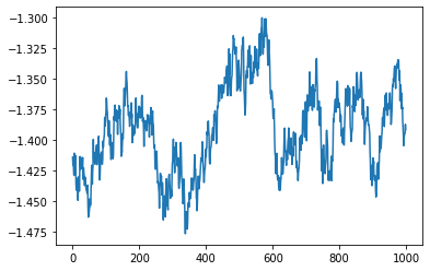
[5]:
plt.plot(samples[:,0])
[5]:
[<matplotlib.lines.Line2D at 0x7fbfbd0d5ee0>]